Data-projects-with-R-and-GitHub

Cross-Study Confidence-Ratings Project

Jakob Raatschen

Confidence Ratings in Three Psychological Studies

For this project we use three datasets from the Confidence database available on the Open Science Framework (OSF). All studies in this database analyse different psychological constructs, but have the same structure concerning their experimental paradigm: Participants are presented with a stimulus and perform some sort of task on it (e.g. determine if they have seen a picture before) for which their performance can be evaluated in a binary fashion (correct/incorrect). Subsequently, they are asked to rate their confidence in their answer.

In this project you are supposed to (1) compare across three studies how confidence relates to the performance of the participants and (2) compare average performance accuracies between studies.

The data sets are not too wrangled, the challenges will be rather to find ways to appropriately compare the studies.

Study 1: Massoni & Roux (2017)

The first dataset is from a study by Massoni and Roux (2017) who tested participants in a perceptual decision making task. You can download the data here. Participants had to decide between two circles which one contained more dots. After each trial they were asked to rate their confidence in their answer on a scale from 0% to 100% with increments of 5%.

Subj_idx	Stimulus	Response	Confidence	RT_dec	RT_conf	Difficulty	Accuracy	Feedback	Study
1	2	1	0.6	1.789951	1.249156	1	0	1	1
1	1	1	0.85	1.296789	2.289089	1	1	1	1
1	2	2	0.95	1.086871	2.472419	1	1	1	1
1	2	1	0.9	1.149476	2.241316	1	0	1	1
1	2	1	0.65	1.266833	1.845008	1	0	1	1

Study 2: Palser et al. (2018)

The second dataset is from a study by Palser et al. (2018) who also investigated confidence ratings in a perceptual decision making task. You can download the data here. Gabor patches were presented in either a first (1) or second (2) interval. Participants had to decide, if they either saw the stimulus in the first or second interval and then rate their confidence in their answer on a scale from 1 to 99 with increments of 1.

Subj_idx	Stimulus	Response	Confidence	RT_dec	RT_conf	Contrast	Condition
1	1	1	22	1.176	2.576	53	Baseline
1	2	2	34	1.094	0.784	53	Baseline
1	2	2	43	0.937	1.256	50	Baseline
1	1	2	34	1.097	1.119	50	Baseline
1	2	2	43	0.917	3.195	53	Baseline

Gabor Patches as Stimuli in Study 2

Study 3: Hu et al. (2017)

The third dataset is from a study by Hu et al. (2017) who investigated memory performance in a recognition task. You can download the data here. In an encoding phase (first presentation of stimuli) a subset of words were presented one after the other. In a subsequent retrieval phase (second presentation of the stimuli) the already shown words were paired with a word that had not been shown before. Participants had to decide which of the two words they had seen before and then rate their confidence in their answer on a scale from 1 to 6. No experimental manipulations (like stimulus difficulty) were applied in this study.

Subj_idx	Stimulus	Response	Confidence	RT_dec	RT_conf	Accuracy
1	1	1	2	2.114	2.006	1
1	1	1	5	1.243	1.94	1
1	1	2	1	3.063	2.298	0
1	1	1	6	1.742	1.421	1
1	2	1	2	3.131	1.339	0

Data Cleaning

Across the three studies the following variables will be in some way of interest: Subj_idx, Stimulus, Response, Confidence & Accuracy (if existing). If for a single study another variable is relevant it will be specifically stated in the following subsections concerning data cleaning.

Study 1

The data set actually contains two studies. We only want to use the second study (Participants 67 to 120), as here no manipulation of the stimulus difficulty (presentation time of stimulus) was applied. Also add a study_id variable that should enable us to identify the distinct study (e.g. Massoni_&_Roux.).

A variable on the Accuracy of the response already exists, so you do not need to create one. However, calculate the average_performance for each participant and add the scores to a separate data frame that also includes a Subj_idx variable as well as the just created study_id variable. This data set will be needed for visualization 2 and should have as many rows as there are participants across all three studies.

Study 2

The variable has a manipulation condition including movement priming. As this mainly impacts the reaction time and we do not investigate that part, you can theoretically ignore this variable. Alternatively, you can only consider the “Baseline” condition, as here no priming occured, making it most comparable to other studies.

There are Nan values (for trials where the response deadline was exceeded). Exclude these trials.

There is a “Contrast” variable, which I assume indicates the contrast of the presented stimuli, however, this is not being explained in the Readme file. For our purposes it should be fine to ignore this variable.

Also add a study_id variable that should enable us to identify the distinct study (e.g. Palser_et_al.).

Add a variable indicating the Accuracy of the participants. For this, you can compare the participants’ answer with the correct answer and assign a value of 1 for correct answers and 0 for incorrect answers. Also, calculate the average_performance for each participant and add the scores to a separate data frame that also includes a Subj_idx variable as well as the just created study_id variable. This data set will be needed for visualization 2 and should have as many rows as there are participants across all three studies.

Study 3

Add a study_id variable that should enable us to identify the distinct study (e.g. Hu_et_al.).

All studies

Because we want to compare the confidence ratings across the studies, we need to obtain a common scale for the confidence ratings. Think about what scale can best be used across studies. This is a bit tricky, to simplify it act as if for study 2 the scale is from 0 to 100 and participants just never indicated a confidence of 0 or 100 (alternative challenge for study 2: for 50% of the confidence ratings at 99 change the score to 100 (the same for 1 and 0), these 50% should be randomly selected. Afterwards think about how to rescale across the 3 studies to have comparable scales). The transformed scales will most likely have its scientific limitations, for our purposes it should be acceptable to look past this.

At this point you should have six dataframes (that is a lot), lets reduce this number:

Concatenate the datasets of the three studies that include the confidence ratings into a single confidence dataset. Variables that should be included are: Subj_idx, Study_id, Accuracy & Confidence (make sure variable names are consistent across the original datasets before concatenating!)

Carefull: Because the studies did not use the same sample of participants we have to distinguish between participants with the same Subj_idx. You could do this for example by adding to the Subj_idx for each participant from study 2 the sample size from study 1 to have no overlap (and keep the variable numerical).

Also concatenate the datasets you have created including the average_performance into a single performance dataset. Again make sure you can distinguish between participants with the same Subj_idx across studies!

Data visualization 1: Confidence ratings and performance accuracy across studies

For this visualization we need the confidence dataset.

The goal should be to create a figure comparing Confidence ratings for correct and incorrect decisions (Accuracy) for each study on both a group and an individual level. For correct decisions confidence should be high, for incorrect decisions low.

On the x-Axis for each study the differentiation between correct and incorrect should be made (Accuracy), the y-Axis should show the Confidence. Label the studies (study_id) based on the colour of the data points/lines and create a legend explaining the colours.

For each study you will need to calculate the average Confidence ratings on an individual and group level for correct and incorrect (Accuracy) decisions.

It could make sense to visualize the data points in a spaghetti plot connecting the Confidence ratings for correct and incorrect decisions for each participant with more transparent lines and the average across all participants with a more prominent line.

If there are any participants that had NO incorrect or NO correct decisions, exclude them for this specific visualization.

Hand Drawn Plot for Visualization 1

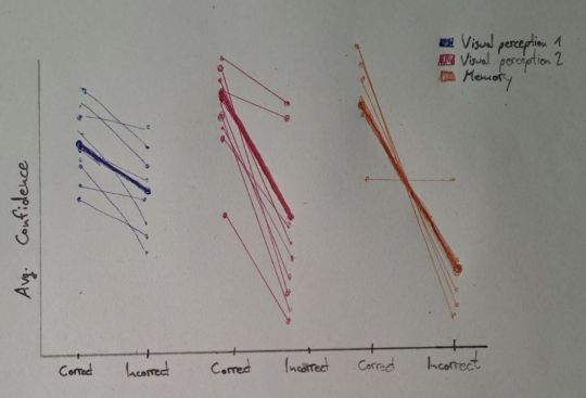
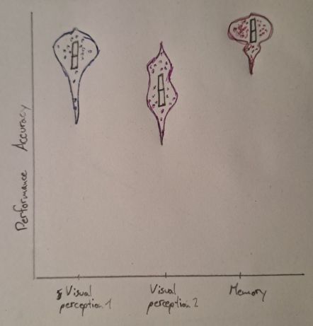
Note: for both visualizations you can choose to either have an x-axis distinguishing between studies (as in the sketches) OR create individual panels for each study. Both alternatives have its advantages, decide what you think makes most sense!

Note II: the studys should be labeled based on the `study_id` variable, the labels here (and in the second visualization) are based on an earlier version.

Data visualization 2: Performance accuracy across studies

For this part we will need a new dependent variable that moves away from confidence ratings and focuses on the actual performance of the participants. For this we need the earlier added average_performance variable (in the performance dataset).

Plot on the x-Axis the study_id and on the y-Axis the average_performance. For the visualization I suggesst violin plots for each study with individual data points (one for each participant) and a boxplot within each violin plot. If you have a reasonable other vision that visualizes the data comparably, feel free to pursue that instead.

Hand Drawn Plot for Visualization 2

References

Hu, X., Liu, Z., Chen, W., Zheng, J., Su, N., Wang, W., … & Luo, L. (2017). Individual Differences in the Accuracy of Judgments of Learning Are Related to the Gray Matter Volume and Functional Connectivity of the Left Mid-Insula. Frontiers in human neuroscience, 11, 399.

Massoni, S., & Roux, N. (2017). Optimal Group Decision: A Matter of Confidence Calibration. Journal of Mathematical Psychology, 79:121-130.

Palser, E. R., Fotopoulou, A., & Kilner, J. M. (2018). Altering movement parameters disrupts metacognitive accuracy. Consciousness and Cognition, 57, 33-40.